3. vDiveR Usage
3.1. R Shiny App
Hint
You may watch the demonstration video on how to utilize vDiveR R Shiny App here!
Upload your aligned FASTA / DiMA (v4.1.1) JSON / JSON-converted CSV output file(s) at the Input Data Description tab of vDiveR. There are five input parameters (Figure. 4):
Host Name: Species name of the organism host to the studied virus.
Size of k-mer: k-mer, a window with size of k, gives us the overview, overall diversity of that particular window. By default, DiMA uses k-mer size of nine to evaluate the viral diversity, with respect to cellular immune response.
Protein Name(s): Name of the protein.
Support Threshold: Support is defined as the number of sequences at a given k-mer position that are free of gaps, unknown or ambiguous nucleotide bases, and amino acid residues. Positions with less than 30 sequences (default) are defined as of low support.
Sequence Type: Nucleotide or amino acid (default) sequence.
Other than that, vDiveR allows user to manipulate display parameters (Figure. 4), such as:
Host Number Selection: Select the number of host studied (one (default) or two hosts). vDiveR supports co-visualization of viral diversity dynamics between two hosts.
Font Size: Font size displayed on the plots.
Line and Dot Size: Line and dot size displayed on the plots.
Protein Names in Order: Determine the order of proteins displayed on plot (Please ensure the protein names provided are the same as the one used in input run!).
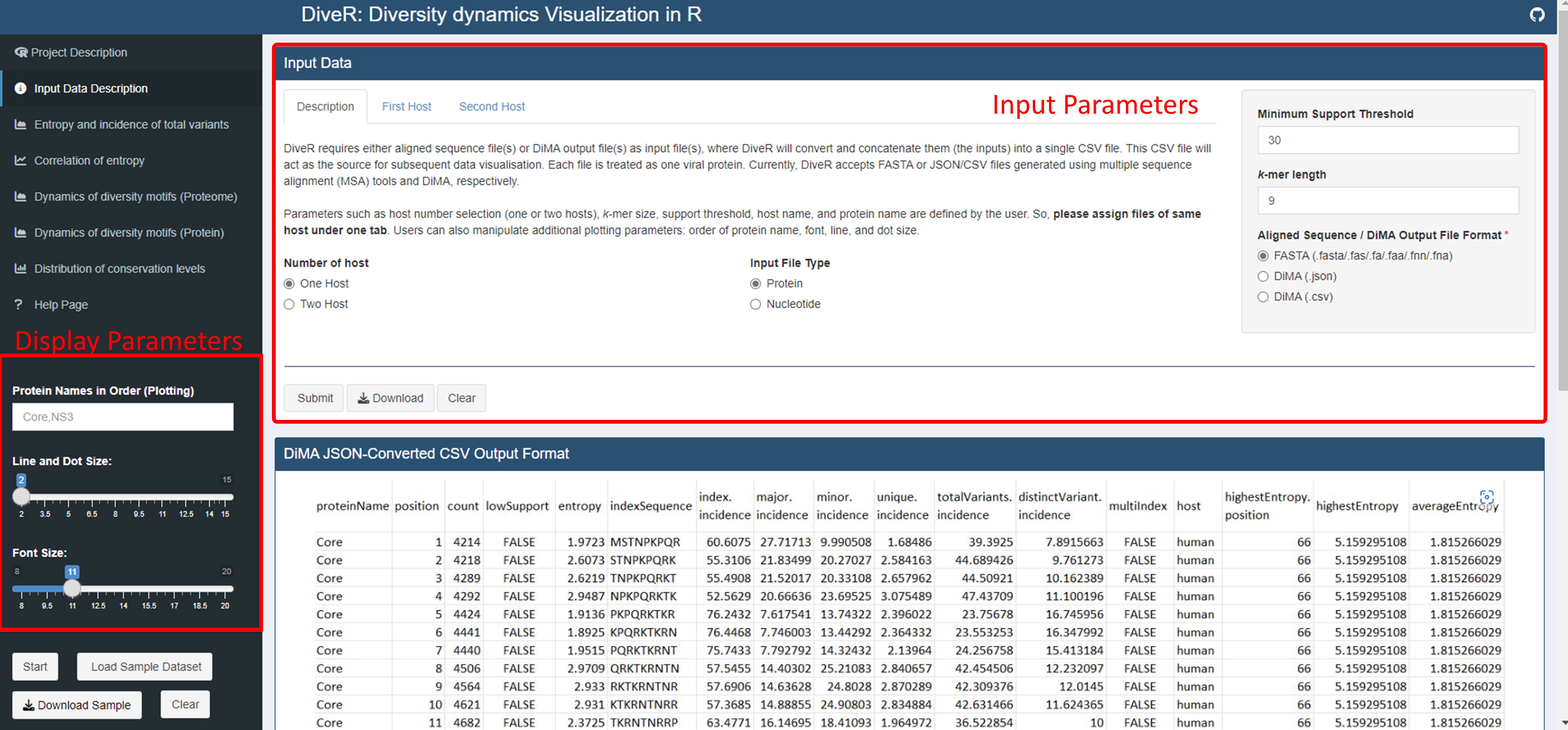
Figure 4. Location of the input and display parameters at vDiveR R Shiny App.
3.2. Bioconductor Package
There are seven functions provided:
json2csv(): convert DiMA (v4.1.1) JSON output to JSON-converted CSV dataframe, which will act as the data source for other functions in vDiveR.
plot_incidence(): plot entropy and total variant incidence.
plot_entropy(): plot entropy.
plot_correlation(): plot correlation between entropy and total variant incidence.
plot_dynamics_proteome(): plot dynamics of diversity motifs at proteome level (not recommended if the studied proteins do not represent the entire proteome).
plot_dynamics_protein(): plot dynamics of diversity motifs at protein level.
- plot_conservationLevel(): plot conservation levels distribution of k-mer positions, which consists of:
completely conserved (index incidence = 100%; black),
highly conserved (90% ≤ index incidence < 100%; blue),
mixed variable (20% < index incidence ≤ 90%; green),
highly diverse (10% < index incidence ≤ 20%; purple), and
extremely diverse (index incidence ≤ 10%; pink).
concat_conserved_kmer(): concatenate completely/highly conserved k-mer positions that overlapped at least one k-mer position or are adjacent to each other and generate the output in dataframe that suits either CSV or FASTA format.
3.2.1. Usage
1.json2csv()
#default arguments
json2csv(json_data, hostName = "unknown host", proteinName = "unknown protein")
#example
inputdf<-json2csv(JSONsample)
Arguments:
json_data: DiMA JSON output dataframe
hostName: name of the host species
proteinName: name of the protein
2.plot_incidence()
#default arguments
plot_incidence(df,host = 1,proteinOrder = "",kmer_size = 9,ymax = 10,line_dot_size = 2,wordsize = 8)

#example 1 (1 host)
plot_incidence(proteins_1host)
#example 2 (2 hosts)
plot_incidence(protein_2hosts, host = 2)
Arguments:
df: DiMA JSON converted csv file data
host: number of host (1/2)
proteinOrder: order of proteins displayed in plot
kmer_size: size of the k-mer window
ymax: maximum y-axis
line_dot_size: size of the line and dot in plot
wordsize: size of the wordings in plot
2.plot_entropy()
#default arguments
plot_entropy(df,host = 1,proteinOrder = "",kmer_size = 9,ymax = 10,line_dot_size = 2,wordsize = 8)

#example 1 (1 host)
plot_entropy(proteins_1host)
#example 2 (2 hosts)
plot_entropy(protein_2hosts, host = 2)
Arguments:
df: DiMA JSON converted csv file data
host: number of host (1/2)
proteinOrder: order of proteins displayed in plot
kmer_size: size of the k-mer window
ymax: maximum y-axis
line_dot_size: size of the line and dot in plot
wordsize: size of the wordings in plot
3.plot_correlation()
#default arguments
plot_correlation(df,host = 1,alpha = 1/3,size = 3,ylabel = "k-mer entropy (bits)\n",xlabel = "\nTotal variants (%)",ymax = ceiling(max(df$entropy)),ybreak = 0.5)

#example 1 (1 host)
plot_correlation(proteins_1host)
#example 2 (2 hosts)
plot_correlation(protein_2hosts, size = 2, ybreak=1, ymax=10, host = 2)
Arguments:
df: DiMA JSON converted csv file data
host: number of host (1/2)
alpha: any number from 0 (transparent) to 1 (opaque)
size: dot size in scatter plot
ylabel: y-axis label
xlabel: x-axis label
ymax: maximum y-axis
ybreak: y-axis breaks
4.plot_dynamics_proteome()
#default arguments
plot_dynamics_proteome(df,host = 1,dot_size = 2,word_size = 15,alpha = 1/3)

#example 1 (1 host)
plot_dynamics_proteome(proteins_1host)
#example 2 (2 hosts)
plot_dynamics_proteome(protein_2hosts, host = 2)
Arguments:
df: DiMA JSON converted csv file data
host: number of host (1/2)
dot_size: dot size in scatter plot
word_size: word size in plot
alpha: any number from 0 (transparent) to 1 (opaque)
5.plot_dynamics_protein()
#default arguments
plot_dynamics_protein(df,host = 1,proteinOrder = "",base_size = 8,alpha = 1/3,dot_size = 3)

#example 1 (1 host)
plot_dynamics_protein(proteins_1host)
#example 2 (2 hosts)
plot_dynamics_protein(protein_2hosts, host = 2)
Arguments:
df: DiMA JSON converted csv file data
host: number of host (1/2)
proteinOrder: order of proteins displayed in plot
base_size: base font size in plot
alpha: any number from 0 (transparent) to 1 (opaque)
dot_size: dot size in scatter plot
6.plot_conservationLevel()
#default arguments
plot_conservationLevel(df,proteinOrder = "",conservationLabel = 1,host = 1,base_size = 11,label_size = 2.6,alpha = 0.6)

#example 1 (1 host)
plot_conservationLevel(proteins_1host, conservationLabel = 1,alpha=0.8, base_size = 15)
#example 2 (2 hosts)
plot_conservationLevel(protein_2hosts, conservationLabel = 0, host=2)
Arguments:
df: DiMA JSON converted csv file data
proteinOrder: order of proteins displayed in plot
conservationLabel: 0 (partial; show present conservation labels only) or 1 (full; show ALL conservation labels) in plot
host: number of host (1/2)
base_size: base font size in plot
label_size: conservation labels font size
alpha: any number from 0 (transparent) to 1 (opaque)
7.concat_conserved_kmer()
#default arguments
concat_conserved_kmer(data,conservationLevel = "HCS",kmer = 9,output_type = "csv")

#example 1 (1 host and store the output in csv format)
csv<-concat_conserved_kmer(proteins_1host)
#example 1 (1 host and store the HCS output in FASTA format)
fasta <- concat_conserved_kmer(protein_2hosts, output_type = "fasta", conservationLevel = "HCS")
#example 2 (2 hosts)
csv_2hosts<-concat_conserved_kmer(protein_2hosts, conservationLevel = "CCS")
Arguments:
data: DiMA JSON converted csv file data
conservationLevel: CCS (completely conserved) / HCS (highly conserved)
kmer: size of the k-mer window
output_type: type of the output; “csv” or “fasta”